Pour commencer, vous pouvez tracer uniquement un sous-ensemble des données. Peut-être sous-échantillonner par un facteur de 4. Bien sûr, vous devrez penser à la méthode de rééchantillonnage qui serait probablement bilinéaire dans ce cas. Qu'en est-il de quelque chose comme la réponse de cette question ici :https://stackoverflow.com/questions/8090229/resize-with-aaving-or-rebin-a-numpy-2d-array
def rebin(a, shape):
   sh = shape[0],a.shape[0]//shape[0],shape[1],a.shape[1]//shape[1]
   return a.reshape(sh).mean(-1).mean(1)

# 1) opening maido geotiff as an array
maido = gdal.Open('dem_maido_tipe.tif')
dem_maido = maido.ReadAsArray()
resampled_dem = rebin(dem_maido, (y/4, x/4))
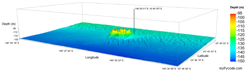
mplot3d est extrêmement lent car il utilise le rendu logiciel. Surveillez votre utilisation de la mémoire et du processeur lorsque vous exécutez ce script, il redlignera un processeur et utilisera 1 à 2 Go de RAM, juste pour rendre un petit raster...
Le sous-échantillonnage ne fera que réduire la qualité/résolution de votre tracé. Une meilleure façon d'accélérer votre tracé consiste à utiliser une bibliothèque de tracés 3D compatible OpenGL, comme Mayavi, qui déchargera le rendu sur votre carte graphique à la place.
Mayavi peut être difficile à installer sous Windows, le plus simple est d'installer une distribution python scientifique comme Anaconda.
Ensuite, vous pouvez utiliser mayavi.mlab.surf au lieu de axes.plot_surface , voir ci-dessous par exemple. La rotation interactive est instantanée.
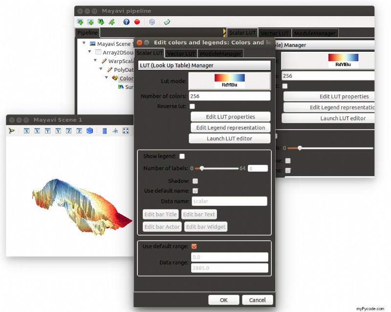
Je vous laisse le soin d'ajouter des axes, de changer de rampe de couleurs et d'ajouter une barre de couleurs (indice, vous pouvez jouer manuellement avec l'intrigue, voir la 2e capture d'écran ci-dessous).
import gdal
#from mpl_toolkits.mplot3d import Axes3D
#from matplotlib import cm
#import matplotlib.pyplot as plt
from mayavi import mlab
import numpy as np

# maido is the name of a mountain
# tipe is the name of a french school project

# 1) opening maido geotiff as an array
maido = gdal.Open('dem_maido_tipe.tif')
dem_maido = maido.ReadAsArray()

# 2) transformation of coordinates
columns = maido.RasterXSize
rows = maido.RasterYSize
gt = maido.GetGeoTransform()
ndv = maido.GetRasterBand(1).GetNoDataValue()

x = (columns * gt[1]) + gt[0]
y = (rows * gt[5]) + gt[3]

X = np.arange(gt[0], x, gt[1])
Y = np.arange(gt[3], y, gt[5])

# 3) creation of a simple grid without interpolation
X, Y = np.meshgrid(X, Y)

#Mayavi requires col, row ordering. GDAL reads in row, col (i.e y, x) order
dem_maido = np.rollaxis(dem_maido,0,2)
X = np.rollaxis(X,0,2)
Y = np.rollaxis(Y,0,2)

print (columns, rows, dem_maido.shape)
print (X.shape, Y.shape)

# 4) deleting the "no data" values
dem_maido = dem_maido.astype(np.float32)
dem_maido[dem_maido == ndv] = np.nan #if it's NaN, mayavi will interpolate

# delete the last column
dem_maido = np.delete(dem_maido, len(dem_maido)-1, axis = 0)
X = np.delete(X, len(X)-1, axis = 0)
Y = np.delete(Y, len(Y)-1, axis = 0)

# delete the last row
dem_maido = np.delete(dem_maido, len(dem_maido[0])-1, axis = 1)
X = np.delete(X, len(X[0])-1, axis = 1)
Y = np.delete(Y, len(Y[0])-1, axis = 1)

# 5) plot the raster
#fig, axes = plt.subplots(subplot_kw={'projection': '3d'})
#surf = axes.plot_surface(X, Y, dem_maido, rstride=1, cstride=1, cmap=cm.gist_earth,linewidth=0, antialiased=False)
#plt.colorbar(surf)  # adding the colobar on the right
#plt.show()

surf = mlab.surf(X, Y, dem_maido, warp_scale="auto")
mlab.show()
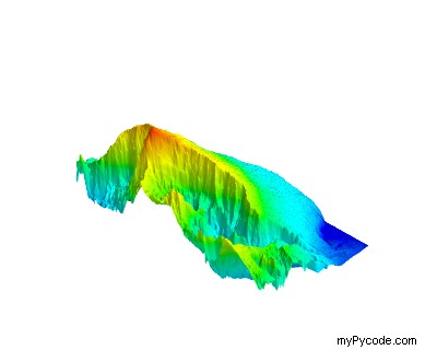
Et un exemple de ce que vous pouvez faire :